Hi everyone! We’re excited to share a quick tour of the headline features landing in Scilab 2026.0.0. This release brings object-oriented programming to the language, new machine-learning utilities, better model exchange in Xcos, and long-requested plotting improvements.
Objects
Scilab now supports first-class objects:
-
classdef … endfor class declarations. -
Constructors, properties, methods, enumeration and operator overloading.
-
Multiple inheritance and well-defined scope/visibility.
Full design notes, guidance, and examples are in the dedicated post: Objects in Scilab
New classification functions
Two widely used clustering algorithms are now built-in:
dbscan(): Density-based clustering that discovers arbitrarily shaped clusters and marks outliers:
rand("seed", 0)
theta1 = 2 * %pi * rand(100, 1);
theta2 = 2 * %pi * rand(120, 1);
theta3 = 2 * %pi * rand(150, 1);

r1 = 1 + 0.2 * rand(100, 1);
r2 = 2.5 + 0.2 * rand(200, 1);
r3 = 4 + 0.2 * rand(300, 1);

X1 = [r1 .* cos(theta1), r1 .* sin(theta1)];
X2 = [r2 .* cos(theta2), r2 .* sin(theta2)];
X3 = [r3 .* cos(theta3), r3 .* sin(theta3)];

N = 10 * (rand(30, 2) - 0.5); //noise

X  = [X1; X2; X3; N];
labels = dbscan(X, 0.72);

f = scf();
f.figure_name = "DBSCAN";
f.figure_size = [975 630];
subplot(122)
gca().isoview = "on";
scatter(X(:,1), X(:,2), [], labels, "fill")
title("Circular cluster with noise");

subplot(121)
gca().isoview = "on";
scatter(X(:,1), X(:,2), [], color(0,127,255), "fill");
title("Raw data");

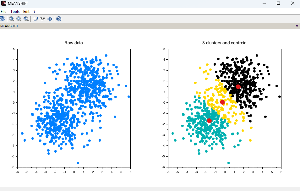
meanshift(): Mode-seeking clustering requiring minimal prior on the number of clusters:
rand("seed", 0);
n = 200;
x1 = rand(n, 2, "normal") + 2 * ones(n, 2);
x2 = rand(n, 2, "normal") - 2 * ones(n, 2);
x3 = rand(n, 2, "normal") * 1.5 + ones(n, 2);
x4 = rand(n, 2, "normal") * -1.5 - ones(n, 2);

x = [x1; x2; x3; x4];

[c, index] = meanshift(x, 2.2);

f = scf(1);
f.figure_name = "MEANSHIFT";
f.figure_size = [975 630];
subplot(122)
scatter(x(:,1), x(:,2), [], index, "fill");
scatter(c(:,1), c(:,2), 150, color(228, 26, 28), "fill"); // centroid of each cluster
title(string(length(unique(index))) + " clusters and centroid");

subplot(121)
scatter(x(:,1), x(:,2), [], color(0,127,255), "fill");
title("Raw data");
Both functions return cluster labels you can pass straight into your plotting pipeline.
Xcos: SSP format support
Xcos now uses SSP format (System Structure & Parameterization) as default format for smoother model exchange with other tools and workflows:
-
Import an existing system description as an Xcos diagram with parameters.
-
Export your diagram and parameters as an SSP package for sharing with other tools.
-
This helps integrate Scilab/Xcos in FMI/SSP-centric environments and toolchains.
Colormaps per axes
You asked, we listened: each axes can now have its own colormap — perfect for side-by-side plots with different palettes.
f = scf();
f.figure_name = "Figure & Axes colormaps";
f.color_map = jet(32);

ax1 = subplot(1, 2, 1);
ax1.title.text = "plot3d() using figure colormap"
x = %pi * [-1:0.05:1]';
z = sin(x)*cos(x)';
e = plot3d(x, x, z, 70, 70);
e.color_flag = 1;


ax2 = subplot(1, 2, 2);
ax2.title.text = "surf() using axes colormap"
ax2.color_map = cool(50);
theta = 0:15:360;
r = 25:5:100;
[R,T] = ndgrid(r,theta);
X = R.*cosd(T);
Y = R.* sind(T);
Z = sinc(R/8);
surf(X, Y, Z)
ax2.rotation_angles=[195 -155];

This removes the old “global colormap” limitation when composing multi-axes figures.
Get involved
-
Try the new features and share your feedback, code snippets, and edge cases.
-
Report issues and suggest enhancements on GitLab.
Thanks to all contributors and testers who helped shape Scilab 2026.0.0!