Ok. There are two facts:
- your (x,y) data is organized on a trapezoidal domain, hence using a rectangular grid to later interpolate will give you (x,y) data outside this domain and thus, extrapolate.
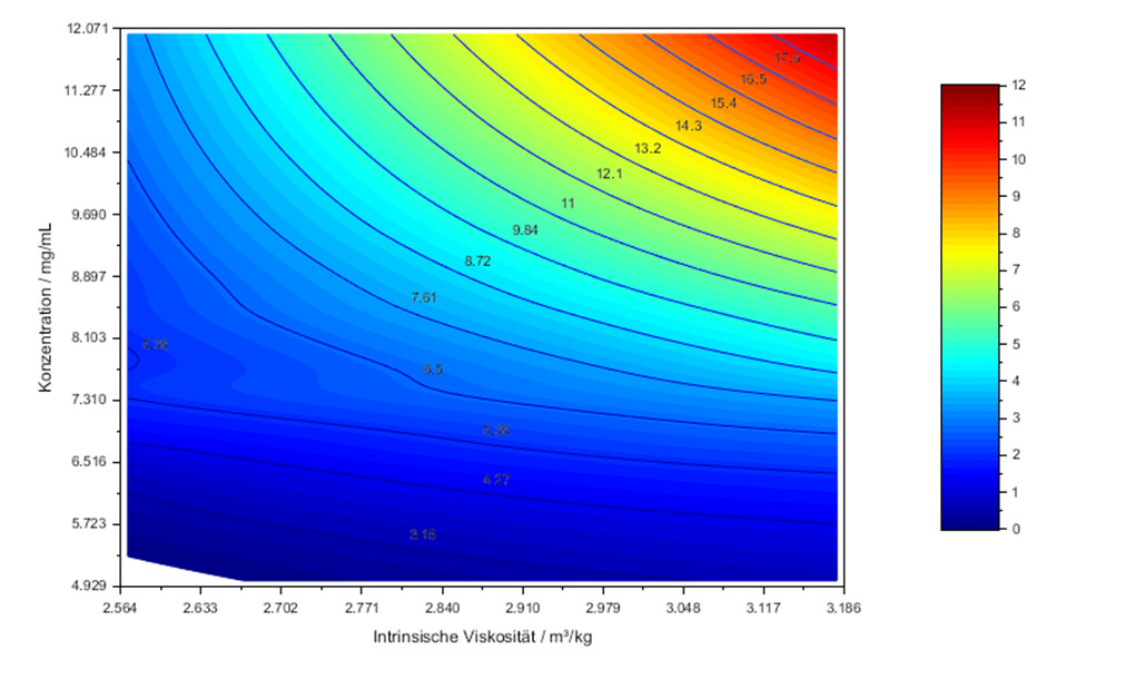
- cshep2d is not well fitted to your (x,y) data: considering the very small number of data points, the cubic interpolation creates artifacts which are irrelevant (see the small “waves” on the left part of your graph above).
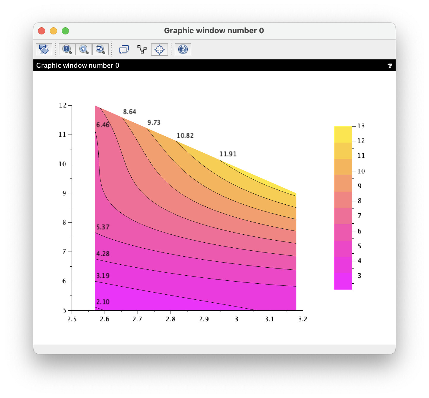
For your data a better approach should be to accept an approximate polynomial model. In the below code, a fine trapezoidal grid is constructed by squeezing a rectangular grid by means of a bilinear transformation, then the z data is fitted w.r.t. a bivariate polynomial constructed on the basis
\{1,x,y,xy,x^2,y^2,xy^2, x^2y, x^2y^2,y^3,y^4\}
You can try other basis but be warned about overfitting ! With the above model the fit is not bad at all
    x      y      z      fitted       error
   ____   ___   _____   _________   _________

   2.57   5     2.04    2.0029712   0.0370288
   2.57   6.5   3.71    3.9171544   0.2071544
   2.57   7     4.785   4.6055525   0.1794475
   2.57   10    6.285   6.2935451   0.0085451
   2.57   12    7.285   7.2857768   0.0007768
   2.96   5     3       3.0398772   0.0398772
   2.96   6     4.3     4.2252302   0.0747698
   2.96   8     8       8.0498465   0.0498465
   2.96   10    11.84   11.825046   0.014954
   3.18   5     3.31    3.31        4.441D-16
   3.18   6.5   5.64    5.64        0
   3.18   9     12.19   12.19       0
and the reconstructed data has no artifact:
I am sorry for the length of the code, but contour lines and pseudo-color plot on a general (non rectangular) mesh are not an easy task in Scilab. Functions to be used are typically:
mesh2d for the generation of the structured triangular mesh,
fec for the pseudo-color plot, and
contour2dm which only computes the contour lines (they have to be drawn and labeled by the user himself):
function mat = model(x,y)
    mat = [ones(x) x y x.*y x.^2 y.^2 x.^2.*y y.^2.*x x.^2.*y.^2 y.^3 y.^4];
endfunction

data=[2.57	5	2.04
2.57	6.5	3.71
2.57	7	4.785
2.57	10	6.285
2.57	12	7.285
2.96	5	3.00
2.96	6	4.30
2.96	8	8.00
2.96	10	11.84
3.18	5	3.31
3.18	6.5	5.64
3.18	9	12.19];

x=data(:,1);
y=data(:,2);
z=data(:,3);

// limits of the (x,y) domain
ymin = 5;
ymax1 = 12;
ymax2 = 9;
xmin = 2.57;
xmax = 3.18;

A = model(x-xmin,y-ymin);
coeffs = A\z;

tab = table([x y z A*coeffs abs(z-A*coeffs)], ...
    "VariableNames",["x","y","z","fitted","error"]);
disp(tab)

// create trapezoidal mesh with a bilinear transformation
[u,v]=meshgrid(0:0.01:1);
tri = mesh2d(u, v);
X = xmin+u*(xmax-xmin);
Y = ymin+v*(ymax1-ymin)+u.*v*(ymax2-ymax1);
X = X(:);
Y = Y(:);
// reconstruct data on mesh
Z = model(X-xmin,Y-ymin)*coeffs;

scf(0)
clf
// change nc set the number of colors/contour lines
nc=11;
// change vmin and vmax to set the first and the last contour line
vmin=2.1;
vmax=13;

gcf().color_map=spring(nc);

// pseudo color plot on mesh
polygons = [1:size(tri,2); tri; ones(1,size(tri,2))]';
fec(X,Y,polygons,Z,zminmax=[vmin vmax],colminmax=[1 nc-1]);
colorbar(vmin,vmax,[1 nc-1]);

// compute and plot contour lines on color plot
[xc, yc] = contour2dm(X,Y,polygons,Z,linspace(vmin,vmax,nc))

k=1;n=yc(k);
while k<size(xc,'*')
  n=yc(k);
  value = xc(k);
  xd = xc(k+(1:n));
  yd = yc(k+(1:n));
  plot(xd,yd,'k')
  [y_max,ind] = max(yd);
  xstring(xd(ind),yd(ind),msprintf("%5.2f",value))
  k=k+n+1;
end